Introduction and Objective

Streamflow discharge is defined as the volume rate of flow of water that includes any substances dissolved or suspended in the water. Discharge is usually expressed in units of cubic feet per second (cfs or ft³/sec). With rare exception, stream discharge is not measured directly, but is computed indirectly from velocity and water level (stage) measurements. If the mean water velocity normal to the direction of flow (V) and the crossectional area (A) of water flow is known, then the discharge (Q) can be computed as Q=VA. As previously discussed in Lesson 1, determining the mean stream velocity is a labor intensive activity, and usually only performed to establish or refine a relationship between stage, which is easy to measure, and discharge. The discharge rating is a relationship between the stage and discharge or between stage, discharge, slope, rate of change of state, or other factors. These relationships are presented in Lessons 7, 8, and 9.

Developing a stage-discharge relationship for a stream requires a set of observed flow (discharge) measurements. Discharge measurements are made at each gaging station to determine the discharge rating for that site. Discharge measurements are initially made are made frequently over a wide range in stages. Periodic measurements are then made (usually monthly) to validate the rating or to identify any changes in the rating caused by changes in the stream channel or stream bed.

The objective of this lesson is to review the techniques and instruments used to measure stream velocity and to calculate stream discharge. The lesson will emphasize discharge measurement via current meters and tracer dilution. We review the methods for determining the vertically averaged velocity at a point and the factors affecting the accuracy of discharge measurement. The interested reader is referred to Rantz et al. (1982) for a review of discharge measurement using the moving boat methodology.

Determining Discharge Using Current Meters

The most common approach to determining discharge is the so called conventional current-meter method. The method is based on determining the mean streamflow velocity and flow cross sectional area; the product of these variables determines the stream discharge. The hydrographer measures stream depth and velocity at selected intervals across a stream's cross section. The hydrographer may be wading, or supported by a cableway, bridge, ice cover, or a boat. Depth and position measurements are made with simple surveying or sounding equipment. A device known as a current meter (described in a section below) measures the stream velocity.

Midsection Method

The USGS currently uses the midsection method of computing stream discharge using current meter velocity measurements. In this method, the stream cross section is divided into rectangular subsections as shown in Figure 5.1. At the center of each of these subsections (called a vertical), a depth and velocity measurement is made, and the distance from a datum point on the shore is determined. The total discharge can be determined using the procedure outlines in Figure 5.2.

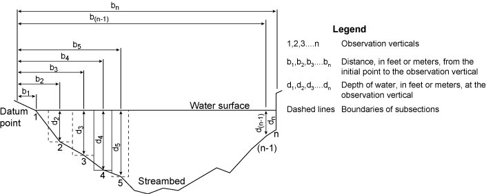Figure 5.1. Definition of terms used in the midsection method.

Figure 5.2. Midsection method development.

The formulas for (q₁) and (q_n) in Figure 5.2 are used whenever there is water only on one side of an observation vertical such as occurs on an island, abutment, or pier. The velocity at an end vertical has to be adjusted as a percentage of the adjacent vertical, since it is not possible to measure the velocity accurately with the current meter close to a boundary. Laboratory data summarized in the table below suggest that the mean vertical velocity in the vicinity of a smooth wall of an idealized rectangular channel is related to the mean vertical velocity at a distance from the wall equal to the depth (V_d).

Table 5.1. Mean vertical velocity near a well as a function of velocity at one channel depth from the well.
Distance from Wall	Mean Vertical Velocity
(Ratio of Depth)	(fraction of V_d)
0.00	0.65
0.25	0.90
0.50	0.95
1.00	1.00

Mean section Method

The mean section method was used by the U.S. Geological Survey prior to 1950. In this older method, discharges are computed for subsections between successive observation verticals. The velocities and depths at successive verticals are each averaged; each subsection extends laterally from one observation vertical to the next. The subsection discharge is the product of the average of two mean velocities, the average of two depths, and the distance between observation verticals. The total discharge is again given by Equation 5.1. Young (1950) determined that the midsection method is simpler to compute and is slightly more accurate than the mean section method.

Measurement Instruments and Equipment used with Current Meter Methods

The purpose of the following sections is to present a brief summary of the more commonly used instruments for the measurement of stream velocity for computing stream discharge using a current meter method. Sections will include a discussion of different types of current meters and miscellaneous other equipment used for depth and position measurements.

Current Meters

A current meter is an instrument that measures the velocity of flowing water. While there are several types of current meters, they all have a blade or cup that spins when the meter is placed in flowing water. The current meter is based on the principle that the velocity of water is proportional to the angular velocity of the meter's rotor. The velocity of water at a given point can be determined by counting the number of revolutions of the rotor during a specified or measured interval of time. The number of revolutions of the rotor is obtained using an electrical circuit through the contact chamber. Contact points in the chamber complete an electrical circuit at selected revolution frequencies. Contact chambers are made that have contact points that complete the circuit twice per revolution, once per revolution, or once per five revolutions. The electrical impulse generates an audible click in the headphones or alternatively, registers a unit on a counting device. The time intervals during which meter revolutions are counted are usually timed with a stopwatch.

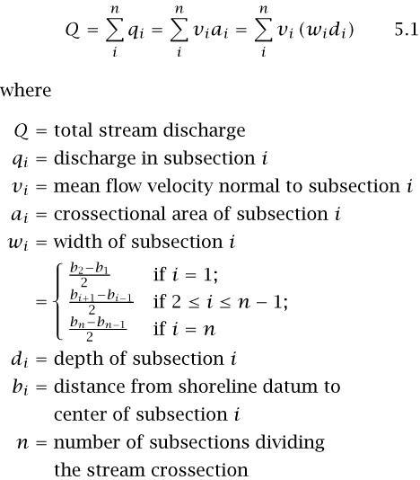
Figure 5.3. Pulsations for two different mean velocities in a 12 foot wide flume (after Rantz, 1982).

Natural streams and artificial channels normally experience turbulent flow. Local eddying always accompanies turbulent flow. Local eddying results in pulsations in the velocity at a point. An example is shown in Figure 5.3 that depicts the pulsations in a laboratory flume for two different mean velocities. Note that the greater the magnitude of the pulsations, relative to the mean at the lower velocity, explains why point current meter observations should cover a longer period when low velocities are being measured. At high velocities, pulsations have a minor impact. Typically, velocities are observed from periods ranging from 40 to 70 seconds. The rational for the interval is based on the observation that pulsations are random. Furthermore, since velocity measurements are made at 25 to 30 verticals, usually with two observation being made in each vertical, there is little likelihood that the pulsations will bias discharge data. Longer periods of current meter observation are not made for two reasons. First, it is desirable to complete a discharge measurement prior to a change in stream stage. And secondly, the use of longer operational periods significantly increases the operating cost of a large number of gaging stations.

Current meters are classified according to their rotors. Vertical-axis rotors, which have cups or vanes, operate in lower velocities than horizontal axis meters. Their bearings are also protected from silty water. The rotor is also repairable in the field without impacting the rating, and the single rotor serves for the entire range of velocities.

In contrast, the horizontal rotor meters disturbs less flow because of the axial symmetry with the flow direction. The rotor is less likely to be entangled with debris, and the bearing friction is less than for vertical axis rotors since the bending moments on the rotor are eliminated.

Vertical Axis Current Meter

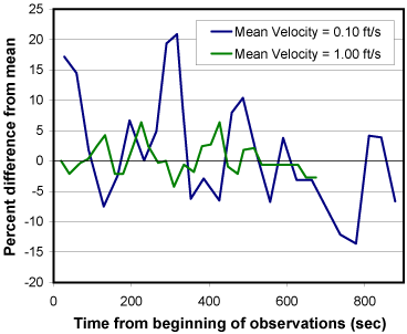
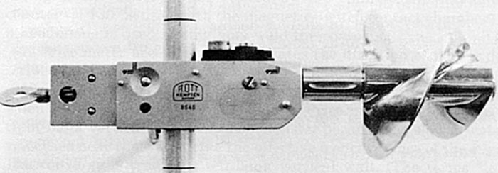
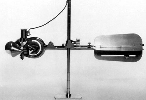
The most common vertical axis current meter used by the U.S. Geological Survey is the Price Meter, type AA (Figure 5.4). The rotor is 5 inches in diameter and 2 inches high with six cone shaped cups mounted on a stainless steel shaft. A type AA meter is also available for low velocities. The low velocity is normally rated from 0.2 to 2.5 cfs. It is recommended for use in streams where the mean velocity at a cross section is less than 1 cfs.

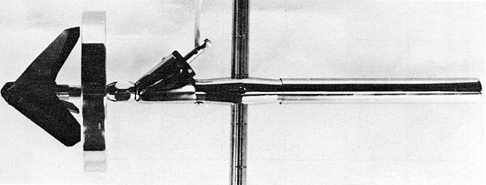
Pygmy current meter are also used in shallow depths (Figure 5.5). It is two-fifths as large as the standard meter. The pygmy meter makes one contact per revolution and is only used with rod suspension

Figure 5.4. Price AA current meter.

Figure 5.5. Pygmy current meter.

A four vane vertical axis meter has also been developed by the U.S. Geological Survey. The instrument is used for measurements under ice cover since the vanes are less likely to fill with slush ice. The instrument has the disadvantage of not responding as well as the Price meter at velocities less than 0.5 cfs.

A limitation of all vertical axe current meters is that they do not register velocities accurately adjacent to a vertical wall. A Price meter located next to a right bank, vertical wall will under-register; the slower water velocities near the wall strike the effective face of the cups. For a left bank, vertical wall, the converse is true. The current meters also under-register when close to the water surface or the streambed.

Horizontal Axis Current Meter

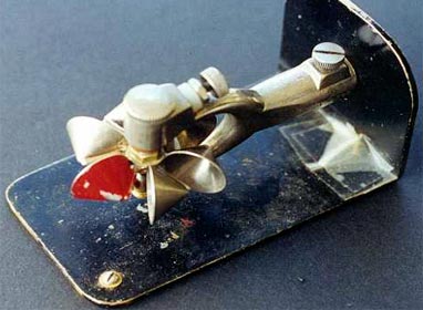
Horizontal axis current meters are the Ott, Neyrpic, Haskell, Hoff, and Braystoke. The Ott meter is made in Germany, the Neyrpic, in France; both are used extensively in Europe. The Haskell and Hoff meters, both developed in the United States, are used in a limited extent. The Braystoke meter is used extensively in the United Kingdom. The Ott meter (Figure 5.6)is not widely used in the United States because of a lack of durability under extreme conditions.

Figure 5.6. Ott current meter..

The Hoff meter (Figure 5.7) is made in the United Sates. It is suited to the measurement of low velocities; it is not appropriate for rugged used.

Figure 5.7. Hoff current meter.

The Haskell meter has been used by the U.S. Lake Survey, Corps of Engineers. It is used in streams that are swift, deep, and clear. A large range in velocities can be measured with the instrument. It is also more durable than other horizontal current meters.

Comparison Horizontal Vertical Axis Current Meters

Townsend and Blust (1960) performed a series of tests to evaluate the performance of vertical axis and horizontal axis current meters. The results indicated virtually identical results from the two meters under favorable measuring conditions (Figure 5.8). The U.S. Geological Survey also conducted a series of discharge measurements on the Mississippi river using Price and Ott meters. The average difference in discharge was -0.15 percent; the Price meter was used as the standard for comparison. The maximum difference in discharge was -2.76 and 1.53 percent.

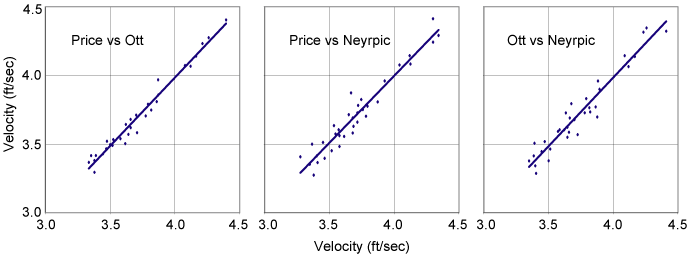Figure 5.8. Comparison of mean velocities measured by Price, Ott, and Neyrpic current meters over a 2 minute period (After Townsend and Blust, 1960).

Optical Current Meter

The U.S. Geological Survey has developed an optical current meter (Figure 5.9). It is designed to measure surface water velocities in open channel without requiring submersion of the equipment. Its primary advantages are for stream environments where the velocities are too high to be measured by a conventional meter, i.e. floods, or where there is significant debris flow that would be hazardous to a current meter.

The meter is essentially a stroboscopic device consisting of a low powered telescope, a single oscillating mirror that is driven by a cam, a variable speed battery operated motor, and a tachometer. The surface of the water is viewed from above through the meter as the speed of the motor is gradually changed to synchronize the angular velocity of the mirror and the surface velocity of the water. Synchronization is achieved when the drift motion on the water surface, as viewed through the meter, is stopped. Surface velocity is computed from the tachometer reading and the meter's height above the water surface.

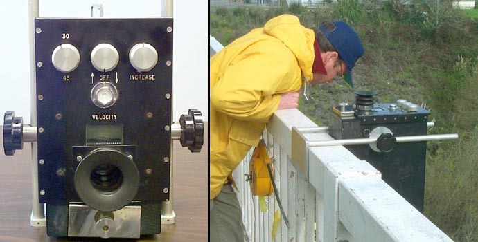Figure 5.9. Optical current meter.

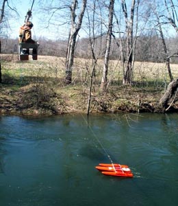
Acoustic Doppler Current Meters

Acoustic Doppler current meters determine stream velocity by measuring the change in sound energy reflected from particles or gas bubbles suspended in the water. Acoustic Doppler velocimeters (ADV) provide point estimates of water velocity, while Acoustic Doppler current profiliers (ADCP) provide velocity estimates in a vertical series of "cells" or "layers" in the water column. ADCPs have an advantage over ADVs since in one operation, ADCPs can provide a complete vertical velocity profile and compute the vertically averaged velocity.

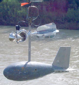
The acoustic Doppler current meters can be mounted on a wading rod, attached to a float and dragged across the river by a cableway (Figure 5.10), or mounted on a boat that is driven across the river (Figure 5.11). The acoustic meters generally can provide 3-D velocity vectors and are usually able to achieve less than 1 percent error over a wide range of flow conditions. The ADCPs can determine the vertical velocity profile in a minute with just one sample setup, and provide a complete discharge computation in the time it takes to sweep, drive, or drag the meter across the channel width. The acoustic Doppler current meters will likely become the standard discharge measurement tool in the near future because of the time savings, accuracy, and relatively low cost.


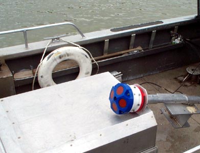Figure 5.10. Acoustic Doppler current profiler on a float attached to hydrographer on a cableway.	Figure 5.11. Boat mounted Acoustic Doppler current profiler.

Additional Measurement Equipment

The use of current meter usually requires the determination of the depth (sounding) and width of the stream. Horizontal position across the stream is generally determined with measuring tapes or marked cables. The depth and position in the vertical are generally measured using rigid rods or via sounding weights suspended from a cable; sonic sounders are also used.

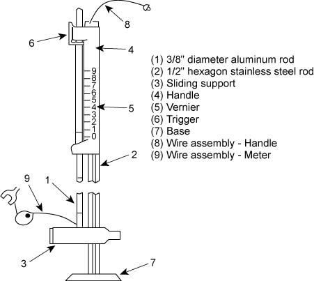
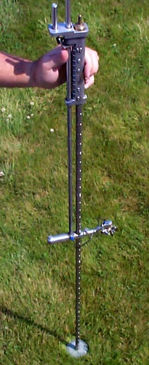
Wading Rods

There are two types of wading rods used for determining depth in a stream. The top setting rod has the advantage of convenience in setting the meter at the proper depth; the hydrographer also keeps his hands dry in the process. The top setting rod has a 1/2 inch hexagonal main rod for measuring the depth and a 3/8 inch diameter round rod for setting the position of the current meter (Figures 5.12 and 5.13). This rod also has a number of design features that assist in setting the current meter at specific fractions (0.2, 0.4, 0.6, and 0.8) of the water depth. As discussed below, these depths are generally used to determine a vertically averaged stream velocity. For example, the current meter is automatically positioned for the 0.6 depth method (or 0.4 depth position measured vertically from the streambed)when the setting rod is adjusted to read the depth of water. When the setting rod is set to read half the depth of the water, the current meter will be positioned at the 0.2 depth position measured from the streambed. Finally, if the setting rod is set to read twice the depth of the water, the current meter will be positioned at the 0.8 depth position measured from the streambed.


Figure 5.12. Top setting wading rod.	Figure 5.13. Top setting wading rod with mounted Price pygmy current meter.

Figure 5.14. Round wading rod with attached Price AA current meter.

The round wading rod has a base plate, lower section, three or four intermediate sections, and a sliding support and a rod end (Figure 5.14). The round rod is used typically in ice measurements. The most convenient length for an ice rod is approximately three feet.

Sounding Weights and Accessories

In streams that are swiftly flowing and too deep to wade, a current meter is suspended in the water by a cable attached to a boat, bridge, or cableway. A sounding weight is suspended below the meter to keep it stationary in the water. The weight also minimizes the damage to the meter when it is lowered to the streambed. The sounding weights are the Columbus weights or C type weights (Figure 5.15). Sounding reels may be used for winding the sounding cables. There are number of types or sizes of sounding reels in common use, with a typical reel illustrated in Figure 5.16.


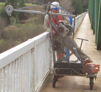Figure 5.15. Sounding weight and Price current meter.	Figure 5.16. 4-Wheel sounding reel crane.

Figure 5.17. Sounding handline.

Discharge measurements from bridges requiring sounding weights that are suspended on handlines (Figure 5.17). They also can be used from cable cars. Handlines consist of an upper or hand cable that is part of the handline used above the water surface. The lower or sounding cable is a light reverse lay steel cable with an insulated core. The sounding cable is tagged at convenient intervals with streams of differing color. These streamers are a known distances above the current meter's rotor. As will be discussed, these tags facilitate the determination of the stream depth.

Handlines have the advantage of ease in assembling the equipment for a discharge measurement. Also it is relatively easy to make discharge measurements from truss bridges that do not have cantilevered sidewalks. The main disadvantages are a lesser degree of accuracy in depth determination, increased physical exertion, and that they can be seldom used for high water measurements of large streams.

Sonic Sounder

An alternative method of determining stream depth is with a portable sonic sounder. The USGS uses commercially available portable depth sounders with a narrow beam angle to minimizes the errors on inclined streambeds and permits the hydrographer to work close to obstructions and piers. Temperature changes affects sound propagation, and the errors is typically plus or minus 2 percent. This error can be reduced by calibrating the sounder with an appropriate average depth determined by other equipment.

Width Measuring Equipment

The distance to any point in a stream's cross-section is measured from an initial point on the stream bank. Discharge measurements are marked at 2, 5, 10, or 20 feet intervals for cableways and bridges. Distance between the markings is estimated or measured with a rule or pocket tape.

Measurements made by wading, in boats or on unmarked bridges. Steel or metallic tapes or tag lines are commonly used measuring devices. Tag lines are made of galvanized steel aircraft cord; solder beads are at measured intervals to indicate distances. The U.S. Geological Survey standard tag lines have beads or tags every 2 feet for the first 50 feet; every 5 feet from stations between 50 and 150 feet; every 10 feet for stations between 150 feet and the end of the tag line.

If the width of the river exceeds 2500 feet, tag lines are impractical. In this case, boats are used to measure the stream width. For example, the boat is lined up with flags positioned on each end of the measurement cross section. The position of the boat in the cross section can be determined by means of a transit on the shoreline and a stadia rod held in the boat. Alternatively, a transit can be set on one bank at a convenient measured distance from and at right angles to the cross section. The position of the boat can be computed by measuring the angle to the boat. In some cases, the position can be determined by electronic distance measuring equipment or by GPS devices. To maintain accuracy, boat measurements are not recommended when there is significant wind and wave action and the stream velocity is less than 1 foot per second.

Vertically Averaged Velocity Determination

Current meters measure velocity at a point in the stream cross section. Discharge measurement requires determining the mean velocity in each of the selected verticals. The mean velocity in a vertical cross section can be approximated by making several velocity observations at different depths and then using a known relationship between these velocities and the vertical mean velocity. Current meters must not be used too close to the surface of the stream bottom to avoid under-registering the velocity. This minimum depth and distance from the bottom is 0.5 feet and 0.3 feet for the Price AA and pygmy meter, respectively. e review the more common methods of determining the mean vertical velocity.

Vertical Velocity Curve Method

In this methodology, a series of velocity observations are made at points distributed between the water surface and the streambed. Normally observations are taken at 0.1 depth increments between 0.1 and 0.9 of the total depth. Observations are always taken at 0.2, 0.6 and 0.8 of the depth to facilitate comparison with other velocity methods.

The vertical velocity methodology is based on plotting the vertical velocities versus the depth. A typical curve is shown in Figure 5.18. Usually, the depths are graphed as fractions of the total depth. The mean velocity in the vertical is obtained by determining the area between the curve and ordinate axis with a planimeter, digitizer, or via numerical integration. The area is then divided by the length of the ordinate axis. Coefficients for the standard vertical velocity curve are shown in Table 5.2.

Figure 5.18. Typical vertical velocity curve.

Table 5.2. Coefficients for standard vertical-velocity curve.
Fraction of total water depth	Ratio of point velocity to mean vertical velocity
0.05	1.160
0.1	1.160
0.2	1.149
0.3	1.130
0.4	1.108
0.5	1.067
0.6	1.020
0.7	0.953
0.8	0.871
0.9	0.746
0.95	0.648

Two-Point Method

The two point methodology uses velocity observations at 0.2 and 0.8 of the depth below the surface. The average of these two observations is the mean velocity in the vertical. The methodology is generally used by the USGS, and has been shown to give accurate and consistent results. The two-point method results are typically within 1 percent of the true mean vertical velocity.

The methodology is limited to depths greater than 2.5 feet when a Price current meter is used. The two point method will also produce erroneous results if, submerged objects or overhanging vegetation in contact with water are, in close proximity to the vertical measuring points. A rough estimate of whether or not the 0.2 and 0.8 depths are sufficient for determining the mean vertical velocity is that the 0.2 depth velocity should exceed the the 0.8 depth velocity but is less than twice as great as the velocity.

Six-Tenths Depth Method

This approach presumes that a velocity observation made in the vertical at 0.6 of the depth below the surface is the mean vertical velocity. Observational data and mathematical models have shown that the 0.6 depth produces reliable results.

The U.S. Geological Survey used the 0.6 depth method under the following conditions:

the depth is between 0.4 and 1.5 feet (Price pygmy meter) or 1.5 and 2.5 feet (Price type AA)
large amounts of slush ice or debris make it impracticable to observe the velocity at the 0.2 depth
the distance between the meter and the sounding weight is too great to place the meter at the 0.8 depth
the stream stage is changing rapidly and a measurement must be quickly made.

Three-Point Method

The three point method is a combination of the two-point and the six-tenths depth methods and utilizes velocity measurements at 0.2, 0.6 and 0.8 of the depth. The mean velocity is determined by averaging the 0.2 and 0.8 depths; the result is then average with the 0.6 depth observation. In equation form, this is

V_mean = (V_0.2 + V_0.8)/4 + (V_0.6)/2 5.2

Occasionally the arithmetic mean of the 0.2, 0.6, and 0.8 velocities will be used instead of Equation 5.2. This method gives more weight to the 0.2 and 0.8 depth observations, and generally produces less reliable estimates of the vertically averaged velocity then does Equation 5.2.

Two-Tenths Depth Method

In the two-tenths depth method, the velocity is observed at 0.2 of the depth of the surface; a coefficient is then applied to the observed velocity to obtain the vertical mean velocity. The two-tenths depth method is not as reliable as either the two-point or the six-tenths depth methods, but it is used in situations where it is not possible to obtain depth sounding or position the current meter at the 0.6 or 0.8 depths.

In lieu of sounding data, a standard cross section can be used to compute the 0.2 depth. The estimation of the 0.2 depth is not critical in the velocity determination since the slope of the vertical velocity curve at this point is nearly vertical (see Figure 5.15).

Normally it assumes each observation 0.2 depth measurement is a vertical mean velocity, and the discharge is then computed using Equation 5.1 without any modifying coefficients. The approximate discharge divided by the area of the measuring section is the weighted mean value of the 0.2 depth velocity. Studies have confirmed that the relationship between the mean 0.2 depth velocity and the true mean velocity remains constant or varies uniformly with stage. The relation may be determined for a particular 0.2 depth measurement by recomputing measurements made at the site by the two-point method using only the 0.2 depth velocity observation as the mean in the vertical. The graph of the true mean velocity versus the mean 0.2 depth velocity for each measurement yields the velocity relation curve, which can be used to correct future two-tenths depth measurement discharge estimates.

Subsurface Velocity Method

In this methodology, the velocity is observed at an arbitrary depth below the water surface. The observed depth should be at least 2 feet below the surface. The method has application when stream stage is available and sounding and depth depth data cannot be estimated reliably. After the stage has receded and soundings can be safely made, the total water depth at each vertical during the earlier measurements can be estimated. The fraction of the total depth of the earlier measurements are also determined by using the depth below the surface measurements of along with the total depth estimates. The coefficients from either the data shown in Table 5.2 or by obtaining vertical velocity curves at the reduced stream stage are used to estimate the mean vertical velocity from the subsurface velocity measurements.

Surface Velocity Method

The surface velocity method is preferable to the subsurface velocity method provided an optical current meter which accurately measures surface velocities is available. In natural channels, a surface velocity coefficient of 0.85 or 0.86 is used to compute the mean velocity. In a smooth channel, the coefficient is 0.90.

Integration Method

In this methodology, the current meter is lowered in the vertical to the streambed and then raised to the surface at a uniform rate. During this time, the total number of revolutions and the total elapsed time are used in conjunction with the current meter rating table to estimate the mean vertical velocity. The method cannot be used with a vertical axis current meter since the vertical movement of the meter affects the motion of the rotor. The methodology is not used in the United States.

Five-Point Method

Another rarely used method in the United States is the five-point method. Observations are make in each vertical at 0.2, 0.6, and 0.8 of the depth below the water surface. Observations are also taken as close to the surface and the streambed as practical. The velocity observations are used to compute the mean vertical velocity, V_mean, using the equation,

V_mean = 0.1( V_surface + 3V_0.2 + 3V_0.6 + 2V_0.8 + V_bed) 5.3

Six-Point Method

The six-point method is also rarely used in the United States. Data points are collected at 0.2, 0.4, 0.6 and 0.8 of the depth below the water surface. The data are supplemented with observations close to the surface and the streambed. The mean velocity is computed from the equation,

V_mean = 0.1( V_surface + 2V_0.2 + 2V_0.4 + 2V_0.6 + 2V_0.8 + V_bed) 5.4

Factors Affecting the Accuracy of a Discharge Measurement

The measurement of discharge is affected by several issues that can bias, distort, and impact the stage discharge relationship. Accurate measurement requires that the measurement equipment be properly assembled and maintained. This is especially critical for current meters which are susceptible to damage.

The underlying characteristics of the measurement section also affects measurement accuracy. Ideally, a cross section lies within a straight reach resulting in streamlines that are parallel to each other. Velocities should be greater than 0.5 feet per second and depths should exceed 0.5 feet. The streambed should also be relatively uniform and free of slack water, eddies, and excessive turbulence. Finally, the measurement section should be located relatively close to the gaging station. Each of these conditions will impact the accuracy of the measurement data.

The spacing of the observation verticals also impacts the measurement accuracy. Ideally, 25 to 30 verticals should be used; the verticals should be spaced so that each subsection will have approximately equal discharge.

If the stage is changing rapidly during measurement, the computed discharge will lose some of its significance. There is also uncertainty as to the representative gage height to apply to the discharge figure. Standard procedures should be shortened with the stage is changing rapidly.

Inaccuracies in sounding and the placement of current meters are most likely to occur in those sections that have great depths and velocities. As a result, heavy sounding weights should be used to reduce the vertical angle made by the sounding weight.

Measurements during freezing winter conditions can be especially challenging. Slush ice interferes with the operation of the current meter's rotor. It also causes difficulty in estimating the effective depth of water. Presuming that the effective depth is that region of the depth where the current meter indicates velocity, the assumed effective depth may be too small if slush ice is interfering with free operation of the rotor.

Wind also affects the accuracy of discharge measurements. Wind can obscure the angle of the current by creating waves that make it difficult to sense the water surface prior to sounding the depth. Wind can also affect the 0.2 depth velocity in shallow water, thereby distorting the vertical velocity distribution.

Carter and Anderson (1963) performed statistical studies that analyzed discharge measurement error in natural streams under average conditions. Four assumptions were evaluated:

the rating of the current meter is applicable to the measurement conditions
the observed velocity is a true time-average velocity
the ratio is known between the velocity of selected points in the vertical and the mean velocity in the vertical
the depth measurements are correct; the velocity and depth are a linear function of the distance between the verticals.

Assumption 1 was evaluated by comparing the ratings from Price current meters when rated in flumes of different sizes. The results indicated that the ratings were repeatable within a fraction of 1 percent.

Assumption 2 was tested in 23 different riverine conditions. The results indicated that the velocity fluctuations were randomly distributed in space and time. If 45 second observations were taken at the 0.2 and 0.8 depths, the standard deviation of the error ratio between the observed and true point velocities was 0.8 percent.

100 stream sites were used to investigate assumption 3. The standard deviation of the error ratios was 1.15 percent.

Finally assumption 4 was evaluated using discharge measurements at 127 stream site with more than 100 verticals were measured in each cross section. For 30 observation verticals, the standard deviation of the error ratios was 1.6 percent. The standard error of a discharge measurement was also computed. For velocity observations of 45 seconds at the 0.2 and 0.8 depths in each of 30 verticals, the standard error was 2.2 percent. The ramification of the results is that if single discharge measurements were made at a number of gaging stations using the methods discussed above, the errors of two third of the measured discharges would not exceed 2.2 percent.

Tracer Dilution Method for Discharge Measurement

An alternative to discharge measurement using current meters is the tracer dilution method. Stream discharge is determined on the basis of how much of the tracer is diluted by the flowing water. Suitable tracers have the following characteristics:

they readily dissolve in water at ordinary temperatures
they are absent in the stream or present at very low concentrations
they are not decomposed in the stream and is not retained or absorbed in significant quantity by plants, sediments, or other organisms
they can be detected in extremely low concentrations
they are harmless to the environment

Salts and dyes have been used in tracer studies. Fluorescent dyes, such as rhodamine, are commonly used tracers for hydrologic studies. Fluorometers are used to measure the concentrations of fluorescent dyes. The fluorometer measures the strength of the light emitted by the fluorescent substance (Figure 5.19).

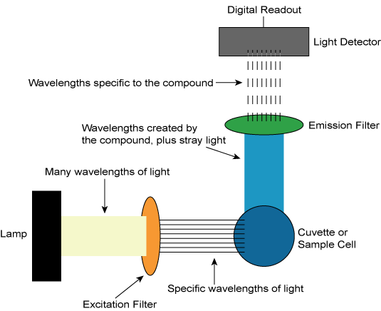Figure 5.19. Basic operation of a fluorometer.

Tracer dilution techniques are more difficult to use than current meter techniques and under most conditions, the results are less reliable. The dilution method should only be used when conditions are unfavorable for current meter discharge measurement, such as in rough channels that exhibit highly turbulent flow.

Theory of the Tracer Dilution Method

In tracer dilution methods, a tracer is injected into a stream and subject to dilution by the stream. The stream discharge can be determined from the rate of injection, the concentration of the tracer in the injection solution, and the downstream concentrations.

There are two primary methods for discharge determination: the constant rate injection method and the sudden injection method. In the constant rate injection method, the tracer solution is introduced to the stream at a constant flow rate over a period sufficiently long to achieve a constant concentration of the tracer in the streamflow and at the downstream sampling locations. The instantaneous injection of a slug of tracer solution is the basis of the sudden injection method. The determination of the total mass of tracer at a sampling cross section determines, indirectly, the stream discharge. Also, if the cross sectional area of the stream or conduit is constant, the sudden injection method may also be used to determine the velocity of flow.

Constant Rate Injection Method

A constant rate injection system is illustrated in Figure 5.20. Provided the tracer is introduced into the stream for a sufficiently long period of time, the concentration variation at a downstream cross section will resemble a concentration time curve similar to Figure 5.21. The stream discharge can be computed using Equation 5.6 developed in Figure 5.22.

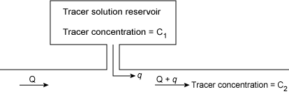Figure 5.20. Constant rate tracer injection system.

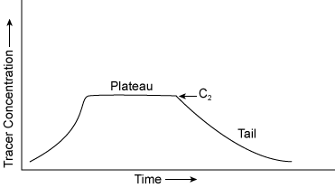Figure 5.21. Typical concentration curve with constant tracer injection.

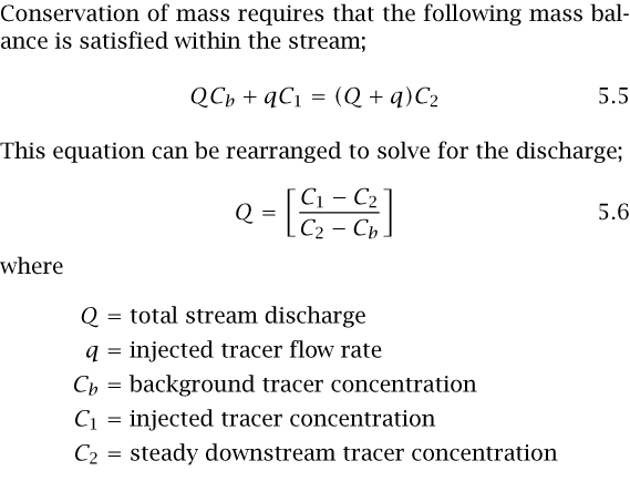Figure 5.22. Equations to calculate discharge for constant rate injection tracer system.

Sudden Injection Method

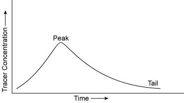
The instantaneous injection of a slug of tracer solution produced a downstream concentration time curve similar to Figure 5.23. The stream discharge can be computed using Equation 5.8 developed in Figure 5.24.

Figure 5.23. Typical concentration curve with sudden tracer injection.

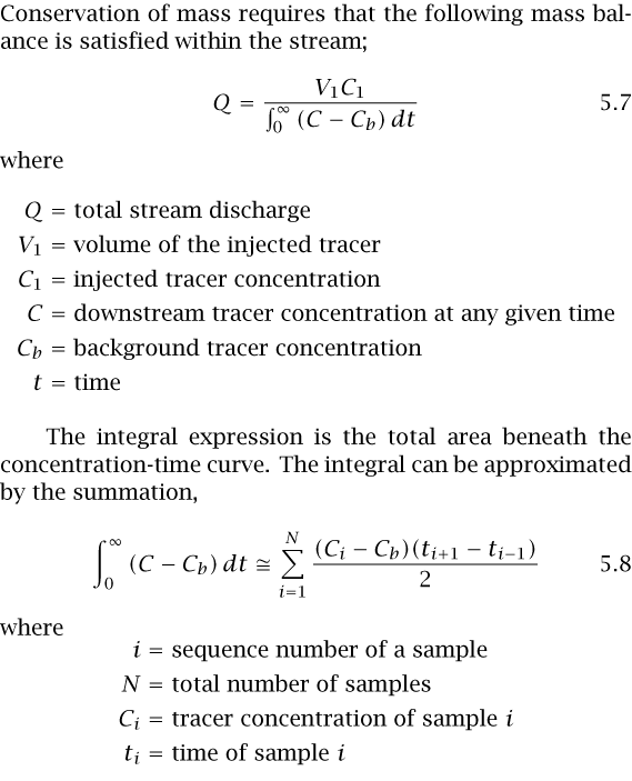Figure 5.24. Equations to calculate discharge for sudden injection tracer system.

Accuracy of the Tracer Dilution Method

There are three primary sources of error in the tracer dilution methodology, turbidity interference, loss of tracer, and insufficient tracer mixing. Turbidity can either increase or decrease the recorder tracer concentrations (fluorescence) depending on the relative concentrations of tracer and turbidity. The effects of turbidity can be minimized by allowing sample to stand long enough to facilitate the settling of suspended solids.

Conservation of mass is the basis for the determination of stream discharge in the tracer dilution method. The accuracy of the discharge calculation is adversely affected if some of the tracer is lost. Tracer losses are typically the result of adsorption and chemical reaction between the tracer and streambed material, suspended sediments, dissolved material in the river water, plants, or other organisms. The amount of tracer loss via adsorption varies primarily with the type of tracer, and the type and concentration of suspended and dissolved solids in the water. The best tracer is that which is least affected by the absorption process.

Photochemical decay is another possible source of tracer loss. It varies with the tracer material used and the residence time in direct sunlight. The losses are usually negligible with fluorescent dyes if the residence time is limited to a few hours.

Examination of Equations 5.6 and 5.7 show that if tracer mass is lost or destroyed by any means between the injection and sample point, the flow will be overestimated. For example, in the sample calculation shown in Figure 5.22, if the downstream concentration of tracer had been recorded as 9 instead of 10 ug/l due to tracer loss, the resulting estimate of stream discharge would be 14.3 instead of 12.5 ft³/sec.

An underlying assumption in the tracer dilution method is the complete vertical and horizontal mixing of the tracer with the ambient fluid. Vertical mixing usually occurs rapidly compared to lateral mixing. As a result, long reaches are typically needed for complete lateral mixing of the tracer. The mixing distance will also vary with the hydraulic characteristics of the reach. It has been shown that ice cover can significantly reduce the mixing capacity of a stream reach (Engmann and Kellerhals, 1974)

In the constant rate injection method, complete mixing has occurred when the concentration, C₂, shown in Figure 5.21 has the same value at all downstream sampling locations. Complete mixing has occurred in the sudden injection method when the area beneath the concentration time curve (Figure 5.23) has the same value at all points in the downstream sampling cross section. In either approach, for a reach of given geometry and stream discharge, the length of time for adequate mixing of the tracer is the same.

Complete or perfect mixing is seldom the goal since it requires an extremely long channel and a long period of injection or sampling. There exists an optimum mixing length for a given stream reach and discharge. If too short a distance is used, there is an inaccurate accounting of the tracer mass as it passes the sampling site. In contrast, too great a distance will produce excellent results but only if it is feasible to sample for an extended period of time. The optimum mixing length is the length that produces adequate mixing for accurate discharge measurements, but does not require an unusually long duration of injection or sampling.

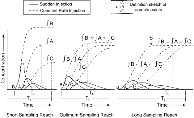
These concepts are illustrated in the Figure 5.25. In the short sampling reach set of curves, adequate mixing occurs, and the tracer cloud must be sampled for its entire time of passage at several lateral locations in the channel, A, B, C. It is generally regarded that at least three sampling points should be used at each sampling site. Also as shown in the Figure 5.25, optimum sampling reach and long sampling reach of curves, the tracer cloud resulting from sudden injection must be sampled at the sampling site from the time of its first appearance there until the time, T_t, of is disappearance from the sampling cross section. In the constant rate of injection methodology, a plateau will first be reached at all points in the cross section at time T_t after injection begins at the injection site. The duration of injection must be at least equal to T_c; injection should continue long enough thereafter to ensure adequate sampling of the plateau. In the long sampling reach, sampling at time S would result in a false conclusion that mixing was poor and the minimum required sample period, T_c, is extremely long. This results in excessive sampling costs.

Figure 5.25. Tracer concentration curves under a variety of injection and sample reach lengths.

The constant rate of injection method has become increasingly popular since reliable injection equipment is available and the sampling process is relatively simple. Provided an injection period is well in excess of T_c, the sampling can be done leisurely at several points in the cross section. The sudden injection method is simple but the sampling process is much more demanding. More reliable results are usually generated by the constant rate of injection method.

Lesson 5 Summary

With rare exception, stream discharge is not measured directly, but is computed indirectly from velocity and water depth (stage) measurements. Determining the mean stream velocity is a labor intensive activity, and usually only performed to establish or refine a relationship between stage and discharge. Discharge measurements are made at each gaging station to determine the discharge rating for that site.

This lesson reviewed the techniques and instruments used to measure stream velocity and to calculate stream discharge. The lesson emphasized discharge measurement via current meters and tracer dilution. The lesson also presented the methods used for determining the vertically averaged velocity at a point and the factors affecting the accuracy of discharge measurement.

The following terms and concepts were introduced in this lesson and should be mastered prior to continuing with on to Lesson 6. Selecting a link in the list below will result in a jump to the portion of the lesson material above that covered the relevant material so that it can be reviewed as necessary.

Definitions
Concepts

Lesson 5 Review Questions

Which two parameters are measured in order to indirectly compute streamflow?
Why are schemes such as measuring current at two-tenths and eight-tenths of the stream depth are used?

Lesson 6 Preview

The discharge rating curve transforms the stage data to a continuous record of stream discharge. The discharge rating curve may be simple or complex depending on the factors or variables considered in the underlying stage discharge equation. Lesson 6 examines simple stage discharge models in which the discharge is only a function of stage. Lesson 6 also describes how these stage-discharge relationships can be extrapolated for other flow conditions.