Introduction

The objective of this lesson is to develop rating curves for a tidal or tidally influenced stream or river. The rating curve can be determined using a combination of a velocity index and stage. In small streams, a deflection meter can be used to obtain continuous velocity records. In larger streams, the acoustic velocity meter is used to determine the velocity index.

The continuous discharge record can also be developed using either models representing steady flow equations for a tidally influenced stream or empirical equations. The appropriateness of the empirical approach is dependent upon the magnitude of the acceleration head. In most situations, mathematical models based on conservation principles are preferable.

Both the theoretical and empirical methods require a recording stage gage at either end of the channel reach. These gages are synchronized in such a way that the simultaneous stage at the two sites can be deduced from the stage records. The approaches also requires discharge measurements for model calibration.

This lesson will address the empirical development of the stage discharge relationship in tidal systems. We begin, however, by illustrating the development of a simplified numerical model of the unsteady flow equation.

Unsteady Flow Equation Numerical Model

The conservation of mass and momentum equations were developed in Lesson 2. Assuming (1) a rectangular channel, and (2) the overall fluid density is constant in the tidal reach, the equations may be expressed as,

∂y ∂t +y  ∂u ∂x +u  ∂y ∂x =0      9.1

∂u ∂t +u  ∂u ∂x +g  ∂y ∂x =g(S0-Sf)      9.2

where y is the depth, u is the velocity in the x direction, g is the acceleration coefficient, S₀ is the slope of the channel bed, and S_f is the friction slope.

Unsteady Flow — Explicit Finite Difference Approximation

The coupled system of mass and momentum equations are commonly approximated using finite difference methods. The most direct method of solving the equations is using a explicit finite difference scheme.

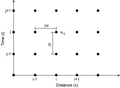
Figure 9.1. Typical finite difference grid in space and time.

In the finite difference method, the continuous representation of the depth, y, and velocity, u are replaced by discrete approximations. Figure 9.1 shows a typical finite difference network in x and t. The solution with finite differences identifies the dependent variables of the flow and momentum equations (the depth and velocity) at the discrete points in the network. Δx and Δt refer to the distance step, the interval between velocity evaluations, and time step. The solution for the velocity and depth is determined for each time step over the modeling or simulation period.

The continuous derivatives in the continuity and momentum equations are replaced by discrete approximations. Defining i as the index of the spatial variable and j similarly for time, the approximations for the derivatives in the continuity and momentum equations can be expressed as:

[  ∂u ∂x ] i,j  =  ui+1,j-ui-1,j Δx      9.3

[  ∂u ∂t ] i,j  =  ui,j+1-ui,j Δt      9.4

[  ∂y ∂x ] i,j  =  yi+1,j-yi-1,j Δx      9.5

[  ∂y ∂t ] i,j  =  yi,j+1-yi,j Δt      9.6

Substituting the approximations in the continuity equation yields

yi,j+1-yi,j Δt +yi,j [  ui+1,j-ui-1,j Δx ] +ui,j [  yi+1,j-yi-1,j Δx ] = 0      9.7

The depth at node i,j+1 can be expressed as

yi,j+1=yi,j+  Δt Δx [ ui,j(yi-1,j-yi+1,j)+yi,j(ui-1,j-ui+1,j)]      9.8

Similarly, the discrete form of the momentum equation can be expressed as

ui,j+1-ui,j Δt +ui,j [  ui+1,j-ui-1,j Δx ] +g [  yi+1,j-yi-1,j Δx ] = g(S0-Sf)      9.9

In unsteady flow problems, the friction slope, S_f, is estimated using either the Manning or Chezy equation. The Manning equation yields,

Sf =  u|u|n2 αR4/3

where R is the hydraulic radius, n is Manning's roughness coefficient, and α is a parameter depending on units. α = 1 in the SI system; in English units, α = 1.49.

The absolute value notation indicates that the frictional resistance always opposes the fluid motion. Assuming a wide, rectangular channel, the discretized form of the friction slope is

Sf,i,j+1 =  ui,j+1|u|i,j+1n2 α2 yi,j+14/3      9.10

Introducing Equation 9.10 into Equation 9.9 yields

ui,j+1-ui,j Δt +ui,j [  ui+1,j-ui-1,j Δx ] +g [  yi+1,j-yi-1,j Δx ] =g [ S0-  ui,j+1|u|i,j+1n2 α2 yi,j+14/3 ]      9.11

Defining

Ψ =  α2 yi,j+14/3 g Δt n2      9.12

then the momentum equation can be simplified to

ui,j+1|ui,j+1| +Ψui,j+1 +Ψ [  ui,jΔt Δx ( ui+1,j-ui-1,j)+  gΔt Δx (yi+1,j-yi-1,j) -gΔt S0 ] = 0      9.13

Equation 9.13 is a quadratic equation in u_i,j+1. The solution can be expressed as

ui,j+1=  -Ψ+ (Ψ2 -4 Ξ)1/2 2      9.14

where

Ξ = Ψ [  ui,jΔt Δx ( ui+1,j-ui-1,j)+  gΔt Δx (yi+1,j-yi-1,j)-gΔt S0 ]      9.15

The depth at node i,j+1 is given by Equation 9.8.

The solution procedure for unsteady flow in a wide rectangular channel consists of the following stages:

1. Discretize the time and spatial domain, i.e. discretize the length of the river into a number of computational elements or nodes, Δx. Similarly discretize the entire simulation period into a number of discrete time periods Δt.
2. Determine the initial depth and velocity in the river. These data, which are known as the initial conditions, correspond to the conditions at t=0. Initial conditions are often represented as uniform or gradually varied flow.
3. Determine the depth, velocity or discharge at the upper and lower boundaries of the channel reach. These are known as boundary conditions. A typical boundary condition is an upstream hydrograph.
4. Solve Equation 9.8 and identify the depth, y_i,j+1.
5. Solve the quadratic equation, Equation 9.13, for the velocity, u_i,j+1.
6. Repeat steps 4) and 5) until the downstream boundary is met; advance the solution over the next time interval and return to Step 3).

The procedure terminates at the end of the simulation period.

The principal limitation of the explicitly finite difference methodology is its stability. It is possible for the numerical errors to amplify during the solution process. A sufficiency condition for the stability of the numerical scheme is the Courant condition,

Δt <  Δx u+c      9.16

where c is the wave celerity. Practical experience suggests that Δt should be about 20% of the value indicated by Equation 9.16.

More stable explicit finite difference solution can be achieved by modifying the finite difference approximations. As discussed by Viessman et al. (1977), the approximations can be expressed as,

[  ∂u ∂t ] i,j  =  ui,j+1-0.5(ui-1,j+ui+1,j) Δt      9.17

[  ∂y ∂t ] i,j  =  yi,j+1-0.5(yi-1,j+yi+1,j) Δt      9.18

Sf=  Sf,i-1,j+Sf,i+1,j 2      9.19

These approximations allow a significant increase in the time discretization, Δt. In addition to the Courant condition, an additional friction criterion must also be satisfied,

Δt <  α2 R4/3 gn2 |u|      9.20

Generally, the minimum of the Courant condition and the friction criterion is used to set the time step, Δt.

Unsteady Flow — Method of Characteristics

An alternative to the explicit finite difference method is the method of characteristics. Again assuming a wide, rectangular channel, the continuity and momentum equations can be rewritten as

A1=  ∂y ∂t +y  ∂u ∂x +u  ∂y ∂x = 0      9.21

A2 =  ∂u ∂t +u  ∂u ∂x +g  ∂y ∂x -g(S0-Sf) = 0      9.22

It is possible to combined these equations with an unknown multiplier, λ, such that

A = λA1+A2      9.23

For any two real and distinct values of λ, two equations in u and y can be produced that have the original properties of the continuity and momentum equations. Combining Equations 9.21, 9.22, and 9.23 yields

A = [  ∂u ∂x (u+λy)+  ∂u ∂t ] +λ [  ∂y ∂x ( u+  g λ ) +  ∂y ∂t ] -g(S0-Sf)      9.24

Recalling the definition of the total derivative, we have

du dt =  ∂u ∂x  dx dt +  ∂u ∂t   provided    dx dt = u+λy      9.25

dy dt =  ∂y ∂x  dx dt +  ∂y ∂t   provided    dx dt = u+  g λ      9.26

Equating the expressions for dx/dt produces,

u+λy = u+  g λ      9.27

and

λ = ± (g/y)1/2      9.28

The two, distinct real roots of Equation 9.28 can be used to transform the equations for A₁ and A₂ into a pair of ordinary differential equation,

du+dy(g/y)1/2+g(Sf-S0)dt = 0      9.29

and,

du-dy(g/y)1/2+g(Sf-S0)dt = 0      9.30

We also require via Equations 9.25 and 9.26,

dx = (u+(gy)1/2 )dt      9.31

dx = (u-(gh)1/2)dt      9.32

Figure 9.2. Method of characteristics solution curves.

Equation 9.31 is known as the positive characteristic curve in Figure 9.2, C+. The negative characteristic curve, C-, is also shown in Figure 9.2.

The solution of Equation 9.29 to Equation 9.32 is again accomplished using finite differences. In this case however the distance step, Δx, and time step, Δt, are variable. Consider the three points in the domain of the problem, A, B, and C. The discretized equations can be expressed:

uB-uA = (g/y)1/2 (yB-yA)+(tB-tA)(Sf,A-S0) = 0      9.33

xB-xA = (uA+(gyA)1/2(tB-tA)      9.34

uB-uC-(g/yC)1/2(yB-yC+(tB-tC)(Sf,C=S0) = 0      9.35

xB-xC=(uC-(gyC)1/2)(tB-tC)      9.36

The length of the variable time step, t_B is obtained by differencing Equation 9.36 from Equation 9.34,

tB =  xA-xC+tC[uC-(gyC)1/2]-tA[uA-(gyA)1/2] uC-uA-(gyA)1/2-(gyC)1/2      9.37

The downstream distance step, x_B is from Equation 9.34,

xB = xA+[uA+(gyA)1/2](tB-tA)      9.38

The flow depth, y_B, is determined by subtracting Equation 9.35 from Equation 9.33 or

yB =  uA-uc+yA(g/yA)1/2+yC(g/yC)1/2+(tB-tc)(SfC-S0)-(tB-tA)(Sf,A-S0) (g/yA)1/2+(g/yC)1/2 = 0      9.39

Finally the flow velocity is

uB = uA-(g/yA)1/2 (yB-yA)-(tB-tA)(Sf,A-S0)      9.40

The method of characteristics was used during the early numerical modeling of the unsteady flow equations. As discussed by Bedient and Huber (2002), the approach is cumbersome primarily because of the interpolation that is necessary for the variable grid mesh. This network of variable grid points, as described in the equations, is determined by the intersection of the positive and negative characteristic curves. Explicit and implicit numerical schemes are far more efficient.

Unsteady Flow — Model Calibration and Validation

The application of a numerical model requires an extensive data base for the stream or river for model calibration. Model calibration involves adjusting the numerical parameters, Δx and Δt, and the hydraulic parameters of the model to achieve the best match between the historical conditions and the model's "predicted" depth and velocity or discharge.

Typically the data base for model calibration will include current meter discharge measurements samples over several tidal cycles at either end of the channel reach. These data are used to determine the resistance and conveyance properties of the reach and to "validate" the computed discharges. The data should include one series made during low freshwater discharge and large tidal range; another should be made during high freshwater discharge. For an unstable alluvial channel, several additional data sets are likely necessary. Enough data are required in either case to define the discharge hydrograph to an accuracy that will permit discharges to be determined at 15 minute intervals over the tidal cycle. Also, the data sampling should be limited to the sections of tidal reaches that are affected by the propagation of long, low-amplitude, translatory waves. These locations are those where there is not a distinct salinity wedge, e.g. variable density.

Empirical Methods

A number of empirical models have been used to develop the rating in tidal reaches. These include

1. the method of cubatures
2. the rating fall method
3. tide correction method
4. coaxial graphical correlation method

The Method of Cubatures

The method of cubatures is based on conservation of mass in tidal estuaries (Pillsbury, 1956). Conservation of mass requires that the outflow at the study station is balanced by the inflow plus or minus the change in storage. The inflow in the continuity equation is the freshwater discharge measured at an upstream gaging station from the head of the tide; the gage station is assumed to have a simple stage discharge relationship. The storage element is the volume of water in the reach between the inflow gaging station and the study station on the estuary. The evaluation of the storage usually requires intermediate gaging stations. The gages are located such that no significant error is introduced by assuming that the water surface is essentially a plane. Usually the differences in the tidal ranges on the opposite shores of a wide estuary can be neglected. Also, the tides at all gaging stations are referenced to the same horizontal datum, usually taken to ensure that all stages are positive.

Freshwater inflow to the reach is estimated if the flow is relatively small. Otherwise, it is necessary to have a continuous record of freshwater inflows.

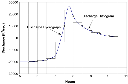
The procedure is illustrated in Table 9.1 for a 5.8 mile reach of the Delaware river. This is the second reach in the estuary; the first reach extends upstream from Trenton to the Delaware river gaging station. As shown by Pillsbury (1966), the total freshwater inflow to the second reach is -12,200 ft³/sec; the downstream or ebb flow is considered negative. The flow is composed of 12,000 ft³/sec of the mainstream and 200 ft³/sec for tributary inflow. The time interval in the computations, Δt is 30 minutes. Note that the numbers in column 9 are obtained from similar upstream computations. Column 10, the summation of columns 8 and 9; the outflow, shown in column 11, is the sum of the total storage change and the total freshwater inflow. Figure 9.3 summarizes the discharge hydrograph for the reach.

Table 9.1. Sample computation of discharge in Delaware River using method of cubatures (after Pillsbury, 1956).
	Tidal Stage						Change in Storage
Time	Upper Station	Lower Station	Mean (y)	Mean Stage	Water Surface Area (A)	Δy	Study Reach	Upstream Reach	Total	Qutflow (Q)
(hr)	(ft)	(ft)	(ft)	(ft)	(1000 ft2)	(ft)	(cfs)	(cfs)	(cfs)	(cfs)
1	2	3	4	5	6	7	8	9	10	11
0500	2.78	2.52	2.65
				2.48	39703	-0.35	-7720	-500	-8220	-20420
0530	2.43	2.16	2.30
				2.12	38880	-0.35	-7560	-490	-8050	-20250
0600	2.09	1.81	1.95
				1.80	38206	-0.31	-6580	-430	-7010	-19210
0630	1.79	1.50	1.64
				1.52	37656	-0.25	-5230	-410	-5640	-17340
0700	1.51	1.27	1.39
				1.59	37800	0.40	8400	20	8420	-3780
0730	1.52	2.06	1.79
				2.52	39686	1.47	32140	2840	35250	23050
0800	3.48	3.04	3.26
				3.77	42247	1.02	23940	1350	25290	13090
0830	4.41	4.16	4.78
				4.66	44053	0.76	18600	1090	19690	7490
0900	5.16	4.93	5.04
				5.36	45478	0.64	16170	920	17090	4890
0930	5.79	5.58	5.68
				5.96	46702	0.55	14270	770	15040	2840
1000	6.32	6.14	6.23
				6.48	47755	0.49	13000	690	13690	1490
1030	6.80	6.64	6.72

Figure 9.3. Discharge hydrograph for method of cubatures example.

The principal disadvantage of the method of cubatures is that it is a cumbersome procedure. Also the calculated discharge are only a rough approximation of the true discharge. This is caused by the large errors that are inherent in computing the storage components of the continuity equation. It is also imperative that the method be checked for consistency to ensure that the continuity equation is actually satisfied.

Rating Fall Method

Provided the acceleration head is negligible, stage fall discharge relations have been successfully used in tidally affected streams. Lesson 8 addressed these issues. The acceleration head is often small when the slope reach is located at the upper end of the estuary near the head of the tide. The rating fall method can only be used at or near these locations.

Tide Correction Method

The tidal correction method is based on the assumption that there is a direct proportionality between the cycling range in stage observed at any two points in a tidal reach. A relation between the mean discharge, for a tidal cycle, to the mean stage can then be developed. The relationship is calibrated by plotting the mean discharge for a tidal cycle, averaged over several individual measurement over the cycle, versus the adjusted mean stage occurring at the base gage. The adjustment applied to the mean stage at the base gage is the difference, D, at the secondary gage between the observed mean stage and the stage assumed to exist under conditions of the least tidal variation. The difference is multiplied by the ratio of the stage range at the base gage to the stage range at the secondary gage. This is applied to the stage at the base gage. The tide correction method is an approximation of the stage resulting from steady flow discharge under the conditions of fixed backwater.

An example of the approach is presented by Parker et al. (1955) for a base gage on the Miami canal that is located 7.6 miles upstream from the ocean. A tide gage on the ocean is the secondary gage. The datum for both gages is mean sea level. The following data are available:

Table 9.1. Stage data for sample tidal correction method problem.
Stage (ft)	Base Gage	Secondary Gage
Mean	2.64	1.61
Maximum	3.18	2.74
Minimum	2.10	0.48
Range	1.08	2.26

The stage correction at the base gage can then be expressed as,

Stage Correction  = D  stage range base gage stage range at secondary gage =1.61 [  1.08 2.26 ] =0.77

The stage correction is always viewed as negative; therefore the gage height = 2.64 - 0.77 = 1.87 feet.

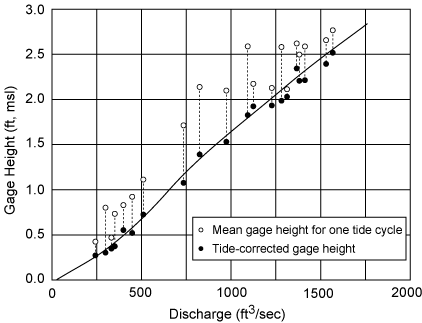
The mean cycle discharge which was determined from 20 set of discharge measurements is plotted versus the actual mean cycle gage heights and the tide corrected gage heights. Figure 9.4 summarizes the data. Although the discharge versus actual mean cycle gage height shows considerable scatter, the discharge-tide corrected gage heights show close agreement. The shape of the rating curve is representative of a stream with a large initial cross section at the point of zero flow.

Figure 9.4. Tide corrected discharge for Miami Canal, FL (after Parker, 1955).

The tide correction method has several advantages. First, it can be used when reverse flows occur during a part of the tidal cycle since the mean discharge of a cycle is used the calculations. Secondly, it is also applicable to a reach of tidal waterway when both observation stations are upstream from the mouth of the waterway. Mean cycle discharge can be graphed versus mean cycle types and the daily mean discharge computed.

The method is generally satisfactory although cumbersome. It has been used extensively in Florida but has seen little application elsewhere in the United States.

Coaxial Rating Curve Method

The coaxial method is a simple procedure for making on site estimates of streamflow. Reading from a pair of stage gages can be used to determine stream discharge directly from a set of rating curves.

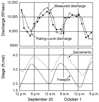
The approach is best illustrated via an example. Coaxial rating curves have been developed for the Sacramento river at Sacramento, California. A total of 302 discharge measurements were made over the period 1957- 1960 (Rantz, 1963). 52 of the measurements provided the baseline data for the curves while the remaining information were used to calibrate and validate the rating curves.

The discharge measurement section is located at the stage recorder in Sacramento. The auxiliary gage is located 10.8 miles downstream. Local inflow is essentially zero, and the stream reach is far enough stream so that flow reversal does not occur. The flow regime is however unsteady for streamflow less that 30,000 ft³/sec. The impact of the tidal effect increases with decreasing upland flow and with an increase in the stage between high and low tides. Stage and discharge data are presented in Figure 9.5.

Figure 9.5. Coaxial rating curve for Sacramento River, Sacramento, CA.

In the development of the rating curve, the dependent variable is the measured discharge at Sacramento. The independent variables include the stage at Sacramento, the fall in the reach, and the algebraic average of the change in stage observed in the reach during a 15 minute interval. The multiple correlation analysis is detailed in Linsley et al. (1949).

The correlation analysis is used to generate a series of curves such as shown in Figure 9.6. First, the curves in the upper left hand corner are used given the stage at Sacramento and the fall in the reach. Next, the curves in the lower left hand corner are entered with the average rate of change in stage. The final step involves the adjustment graph where the discharge is actually read. The adjustment graph is an adjunct to the correlation analysis; it is added to introduce a necessary curvilinearity to the relationship. It also functions in another way by eliminating the need to redefine the other curves if the underlying relationship should change. In this case, only the adjustment curve has to be redone.

Figure 9.6. Adjustment graphs for coaxial rating curve method applied to the Sacramento River, Sacramento, CA.

The validation of the approach on the Sacramento river indicated that 95% of the measurements agreed within ±15% of the rating. The coaxial approach was weakest during those times when the acceleration head is relatively significant.

Lesson 9 Summary

The discharge in many coastal streams experience tidal influence during some portions of the year. Developing rating curves for these streams is important since they are frequently the streams that experience seasonal flooding and resulting property damage. This lesson addressed the empirical development of stage discharge models for tidally influenced stream and a simplified numerical model of the unsteady flow equations.

The following terms and concepts were introduced in this lesson and should be mastered prior to continuing with on to Lesson 10. Selecting a link in the list below will result in a jump to the portion of the lesson material above that covered the relevant material so that it can be reviewed as necessary.

• Definitions
  • Courant condition
• Concepts
  • numerical model for the unsteady open channel flow equations
  • finite difference numerical solution technique for unsteady flow equations
  • method of characteristics solution technique for unsteady flow equations
  • method of cubatures
  • method of rating fall
  • tide correction method
  • coaxial graphical correlation method

Lesson 10 Preview

The material presented in Lessons 1 through 9 introduced the theory and practice of developing stage discharge curves. Lesson 10 will serve to tie all of these concepts together as they specifically relate to NWS hydrologists. Specifically, the lesson will explore methods of estimating stage-discharge relationship for flows that exceed rating curve and how those estimates effect the public forecast products of NWS hydrologists.