Introduction

In the previous lessons we have discussed and reviewed various rating curve models for both natural and artificial control. In practice, ratings curves are often extended or extrapolated beyond the range of discharge measurements. The extrapolation of the rating data can lead to considerable uncertainty in the prediction of discharge. The objective of this lesson is to examine low flow and high flow extrapolation and to quantify possible shifts in the stage discharge relationship.

Low Flow Extrapolation

Low flow extrapolation of rating curves is often required in the management of surface water supply for domestic, industrial, or agricultural uses. Although low flow extrapolation can have important consequences, it is not an area of particular concern to NWS hydrologists.

Low flow extrapolation is performed using rectangular coordinate graph paper since the coordinates of zero flow can not be plotted on the log graph paper. An example of the extrapolation is illustrated in Figure 7.1. The extrapolation is self-explanatory. A curve is drawn between the plotted points at gage heights 0.09 feet and 0.28 in such a way so as to merge smoothly with the rating curve exceeding 0.28 feet.

In most cases, low flow extrapolation is not very accurate. If the existing trend in the rating curve is extended to the zero discharge point, the curve will rarely pass through the zero stage point. Forcing the rating curve through the zero/zero stage-discharge point usually requires a different shaped curve then in the observed portion of the rating curve. Under these conditions, an adequate understanding of the relationship between low stage and discharge can only be achieved with additional low flow discharge measurements.

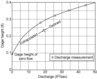Figure 7.1. Rating curve extrapolation.

High Flow Extrapolation

The ramifications of high flow extrapolation are potentially more severe than low flow extrapolation. As discussed in Lesson 1, errors in high flow extrapolation can underestimate flood peaks with the consequent loss of human life and property. Five methodologies are used for high flow extrapolation:

indirect determination of peak discharge
conveyance-slope method
area comparison of peak runoff rates
step backwater method
flood routing

As a general rule and only as a last resort, should the rating curve be extrapolated beyond a discharge that is twice the greatest measured discharge. In the event the extrapolation is required, the hydrologist should identify the upper end of the rating curve using methodology 1, the indirect determination of peak discharge. If this proves infeasible, the other methodologies are used.

Indirect Determination of Peak Discharge

The methodologies discussed in Lesson 5 involve the direct sampling of the stream system. During floods, however, it is usually impractical to assess the peak discharge, especially when roads are impassable, or structures for current measurements no longer exist or are viable.

Indirect measurement of discharge utilizes the energy equation for computing streamflow. The conservation of energy equation for a stream or river is the basis for the development of equations describing open channel flow, flow over dams, and flow through culverts. All the equations, however, involve,

the physical characteristics of the channel
the water surface elevations at the time of peak stage; this is used to define the upper bound of the cross sectional areas and the differences in elevation between two or more significant cross sections
hydraulic factors such as roughness coefficients and discharge coefficients

The data requirements for application of these methods require a field survey of a channel reach. The survey includes the elevation and location of high water marks, cross sections of the channel along the reach, and a description of the geometry of dams, culverts or bridges. Further information on these methods may be found in Benson and Dalrymple (1967), Bodhaine (1968), Dalrymple and Benson (1967), and Hulsing (1967).

Slope-Area Method

The slope-area method is the most common method for indirect discharge calculations. The discharge is computed from the uniform flow equation involving the channel characteristics, water surface profiles, and a roughness or retardation coefficient. As shown in Figure 7.2, the change in the water surface profile represents energy losses caused by bed and bank roughness.

Figure 7.2. Slope-Area method definitions.

In the slope-area method, the discharge, Q, is computed from the uniform flow equation. Recall that the discharge is dependent on the cross sectional area, the hydraulic radius, and the channel slope. In uniform flow, the channel slope is parallel to the energy gradient or friction slope. The friction slope, in turn, can be determined from the energy equation for a reach between any two cross sections. The flow rate can then be computed from these variables.

Uniform flow can be described by Manning's equation,

Q=(δ/n)[AR^2/3S^1/2] 2.28

where δ is a unit conversion factor; δ = 1, SI units and δ = 1.46, for English units. Q is the discharge, A is the cross sectional area, R is the hydraulic radius, S is the channel slope and n is the roughness coefficient. Manning's equation presumes uniform flow in which the water surface profile, S_W, channel slope, S₀, and energy gradient, S_f are parallel to the streambed and the hydraulic radius, area, and depth are constant throughout the reach, e.g. S_W = S_f = S₀ = S.

The energy equation for a reach of a nonuniform channel between two cross sections, 1 and 2, can be expressed as

(h₁+h_v₁)=(h₂+h_v₂)+(h_f)_1-2+k(Δh_v)_1-2 7.1

where h is the elevation of the water surface, h_v is the velocity head, h_f is the energy loss due to boundary friction, Δh_r is the change in the velocity head (upstream minus the downstream), and k is an energy loss coefficient. The friction slope, S_f, can be estimated as

S_f = h_f/L = [Δh + Δh_v - kΔh_v]/L 7.2

where Δh is the difference in water surface elevations between the cross section, and L is the length of the stream reach. The conveyance, K_i, for cross section i is computed as

K_i = (δ/n)[AR^2/3] 7.3

Combining the equations, the discharge can then be expressed as

Q = [K₁K₂S_f]^1/2 7.4

where S_f is the friction slope.

Contracted Opening Method

Roadway crossings contract stream channels and cause an abrupt drop in water surface elevations. The contracted section framed by an abutment and the channel bed acts, in a sense, as a discharge meter. The head on the contracted section is defined by high water marks; field surveys define the geometry of the channel and the bridge.

The drop in water surface levels between an upstream section and the contracted section is a function of the change in velocity. The discharge is dependent on the change in the water surface elevation, the velocity head, and the friction loss.

The contracted opening method is based on the discharge equation,

Q = CA₃[2g(Δh + αu²/(2g) - h_f]^1/2 7.5

where Q is the discharge, g is the gravitational acceleration constant, C is a coefficient of discharge based on the geometry of the bridge and embankment, A₃ is the gross area of the minimum section parallel to the constriction and between the abatements, Δh is the difference in water surface elevations, αu²/(2g) is the weight velocity head, α is a coefficient that takes into account the variation in the velocity, and h_f is the friction loss as determined from the Manning's equation.

Flow over Dams and Weirs

The peak discharge over a dam or weir is determined from a field survey of high water marks and the geometry of the structure. The underlying flow equation is

Q=CBH^3/2 7.6

where Q is the discharge, C is a coefficient of discharge, b is the width of the dam/weir normal to the flow direction, and H is the total energy head.

The reliability of the equation is primarily dependent on the coefficient, C. Values of C vary with the geometry of the dam and the degree of submergence of the dam crest by the tailwater. The reader is referred to Hulsing (1967) for additional information.

Flow through Culverts

The flow through culvert is conceptually similar to flow through dams or weirs. Again the peak discharge can be determined from high water marks defining the headwater and tailwater elevations. The methodology is used to measure flood discharge of small drainage areas.

The location of roadway fill and culvert in a stream channel causes an abrupt change in the flow's character. The channel transitions results in rapidly varied flow dominated by acceleration rather than boundary friction. The flow in the approach channel to the culvert is typically uniform and tranquil. Within the culvert itself, the flow may be tranquil, critical, or rapid; if the culvert is filled, it may flow under pressure.

The peak discharge through a culvert is determined by application of the energy and continuity equations between the approach section and the culvert barrel. Bodhaine (1968) discusses a variety of methods, including trial and error for the computation of the peak discharge in culvert flow. Methods are also available for determining peak discharge in highly sinuous, steep canyon streams. The interested reader is referred to Apmann (1973) for a detailed description of these methods.

Conveyance Slope Method

The conveyance slope method is based on Manning's equation, expressed in terms of the conveyance, K, as

Q=KS^1/2 7.7

where the conveyance is K=(δ/n)AR^2/3, where δ is a conversion factor for English or metric units. Values of A and R for a stream stage can be obtained from a field survey of the discharge measurement cross sections and values of the roughness coefficient, n, can be estimated in the field. As a result, the conveyance can be determined for any given stage. The gage height versus the conveyance can be plotted on rectangular graph paper; a best fit curve can be plotted to the data using any one of a number of standard software packages, including spreadsheet programs such as Excel.

The energy gradient or slope, S, is usually not available even for measured discharges. However from Equation 7.7, S can be obtained as

S=Q²/K² 7.8

The gage height versus S can be plotted for measured discharges on rectangular graph paper. A curve is again fitted to the plotted points, and then extrapolated to the required gage height. The extrapolation is tempered by the fact that at higher stages S tends to become constant and equal to the normal slope of the streambed. If the upper end of the gage height versus S curve shows a constant or nearly constant value of S, the extrapolation is fairly reliable. The discharge for any particular gage height is attained using Equation 7.7, i.e., multiplying the corresponding K value by the square root of the corresponding S value from the S curve.

Errors in the roughness coefficient will have a minor impact on discharge evaluation. The reason for this is that errors in computing K are offset by a similar percentage error in the opposite direction in computing the square root of S. The result is that the errors in each term cancel when multiplied. The exception to this occurs if the gage height S curve has not reached a stage value such that S is nearly a constant. Extrapolation in this case is subject to error. In this event, the slope of the streambed, usually determined from topographic data, provides a more reliable estimate of the constant value of S at high stages.

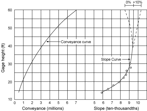
An example of the conveyance slope method is shown in Figure 7.3. The values of K, the conveyance, are computed from the geometry of the measurement cross section. The actual discharge measurements are represented as circles in Figure 7.3; they are defined at a gage height of 60 feet. The gage height slope curve also depicts the error at a gage height of 60 feet, plus or minus 10 percent. The implication is that the error in the discharge reduces to plus or minus 5 percent. The high degree of accuracy is probably the exception in discharge calculations. Note also that the negative error (dashed) curve that shows a decrease in slope at high stages, is potentially greatest when overbank flow occurs.

Figure 7.3. Sample slope-conveyance method results.

The reliability of the conveyance slope method is predicated on a number of important assumptions. First, the methodology assumes the geometry of the cross section is representative of a long reach of a downstream channel. This of course eliminates gaging stations where discharge measurements are made at constricted cross sections, e.g. bridges and cableway measurement stations.

Secondly, the methodology presumes that the slope tends to become constant at higher stages. These conditions of uniform flow are theoretically met only in long, straight channels of uniform cross sections. Natural channels that satisfy these required conditions are virtually nonexistent. As a result, the slope stage relationship need not be vertical at the upper stages. In Figure 7.3, the dashed lines represent the probable error of the discharge calculations. If the two highest discharge points had not been available, it would have been impossible to locate the upper end of the curve with any degree of reliability. A mitigating factor in the calculations is that even with an error of 40 percent in the value of the slope at the upper end of the curve, the error in discharge is only 18 percent or -23 percent depending on whether the estimate was high or low.

Areal Comparison of Peak Runoff Rates

Correlation techniques are often used by hydrologists to relate peak discharges to watershed areas. Assuming flood stages are produced over a large area by an intense storm, the peak discharges can be estimated at gaging stations were they are unknown from the known peak discharges at surrounding stations. The known peak discharges are usually converted to peak discharge per drainage area.

Provided there is little difference in storm intensity of the affected area, the peak discharge per unit area can be correlated with only the drainage area. In the event of variable storm intensity, other index variables are used in the correlation analysis, e.g. the maximum 24 hour basinwide storm precipitation. An example is shown in Figure 7.4.

Figure 7.4. Areal correlation method for peak runoff estimation.

These data are additional information that can be used to extrapolate the rating curves. However, it is important to stress that the underlying principles of extrapolation of log rating curves are not to be violated even with this new information.

Step Backwater Method

In the step backwater method, the water surface profiles for selected discharges are determined via successive approximations. The methodology is initiated at a cross section with a known stage discharge relationship; the method then process to the gaging site which requires extrapolation. If the flow is subcritical, a natural occurrence in streams, the computations proceed upstream. The computations proceed downstream for supercritical flow. The discussion assumes the common situation of subcritical flow.

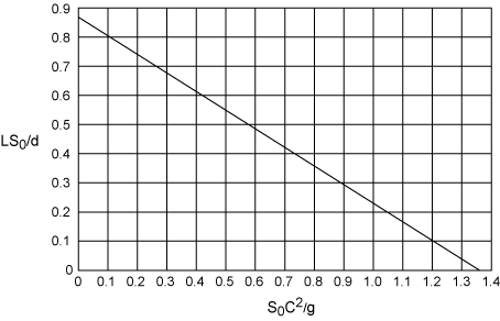
In subcritical flow, the water surface profiles converge upstream to a common profile. If an initial cross section for the computation is selected far enough downstream from the gage, the computed water surface elevation at the gage site will have a single value regardless of the stage selected for the initial site. Figure 7.5 illustrates the relationship between the required distance, L, and stream parameters. The relationship is summarized by the equation,

LS₀/d=0.86-0.64 (S₀C²/g) 7.9

where S₀ is the bed slope, d is the mean depth for the smallest discharge considered, g is the acceleration of gravity, and C is the Chezy coefficient. This assumes that a rated cross section is not available downstream from the gaging site.

Figure 7.5. Relationship between required sample distance (L) and stream parameters for step backwater method.

Once the initial site is selected, the reach is discretized into a number of subreaches. The subreaches are determined by selected cross sections where there are major breaks in the high water profile caused by variation in the channel geometry or roughness. The cross sections become the end of the subreaches. Field work is required to survey the cross sections and estimate roughness coefficients.

Next a discharge, Q, is selected; the stage is then obtained at the initial section with this value of discharge. If the initial section is rated, the stage will be known. If it is not, the estimated stage is computed from the estimated mean depth d. d is estimated from a modified form of the Chezy equation,

d=Q²/[(CA)²S₀] 7.10

where C is again the Chezy coefficient, A is the cross sectional area corresponding to d, and S₀ is the bed slope or water surface slope.

The step backwater calculations are begun at the subreach furthest downstream. Known here is the estimated stage for the value of Q under consideration. The objective of the computations is to determine the stage at the upstream end of the subreach that is compatible with Q. The subreach equations are steady-flow equations, e.g. Chezy or Manning equations. These equations are modified to reflect the nonuniformity in the subreach by the use of the difference in the velocity head at the end cross sections (see the slope area method). The Chezy and Manning equations are related by the equation,

C=(δ/n)R^1/6 7.11

where n is Manning's roughness coefficient and R is the hydraulic radius.

The difference in water surface elevation (Δh) between upstream (1) and downstream (2) cross sections can be expressed as

Δh = h₁ - h₂ = ΔLu₁u₂C^-2R₁^-1/2R₂^-1/2 + (α₂u₂² - α₁u₁²)(1 + k)/(2g) 7.12

where h is the stage, ΔL is the subreach length, and g is the acceleration of gravity. k is a constant, with value zero when α₂u₂² > α₁u₁², and a value of 0.5 otherwise.

α is the velocity head coefficient. It is dependent on the velocity distribution in the cross section (see Equation 2.20). In the United States, the value of 1.0 is used for simply shaped cross sections. More generally, the value of α is given by the equation

α = [∑K_i³/A_i²]/[K_T³/A_T²] 7.13

where A_i is the area of subsection i, A_T is the total area, K_i is the conveyance of subsection i, and K_T is the total conveyance. Formally

A_T = ∑A_i      7.14
K_i = CA_iR_i^1/2      7.15
K_T = ∑K_i      7.16

The calculation of the discharge is an iterative procedure. A trial Q is selected for an upstream cross section. Values of A, u, and R are determined for the upstream and downstream sections. These values are then used to determine Δh, the difference in water surface elevations between the upstream and downstream locations using Equation 7.12. The computed value of Δh is compared with the difference between the trial value of the stage at the upstream cross section and the known or assumed known downstream stage. If they do not agree, which initially is usually the case, a second trial stage value at the upstream cross section is selected. The procedure is repeated; the newly determined Δh is compared with the corresponding trial value. The calculations are repeated until the difference between the computed Δh is less than some prescribed tolerance.

Once this has been accomplished for the subreach, the cross section becomes the downstream cross section for the next subreach upstream. The computations are repeated for that subreach and for each succeeding subreach. Ultimately, the water surface profile will extend to the gaging station that is applicable to the discharge value being studied.

Provided the stage corresponding to the discharge at the initial cross section is known, the stage computed for the gage is viewed as satisfactory. Otherwise, the computations are repeated twice using other values of stage at the initial cross section for the same discharge Q. This ensures consistency of the water surface profiles at the gage. The computations are repeated with an initial stage that is 0.5 to 1.0 feet higher than originally used; then an initial stage approximately 0.5 to 1.0 feet lower is used. The three sets of computations should produce nearly identical values of stage at the gaging station for the discharge Q. In the event they do not, the initial cross section should be moved further downstream and the computations repeated. The entire process is then repeated until data are sufficient to define the high water rating for the gaging station.

Flood Routing

Flood routing methods are another alternative for high flow extrapolation. All the observations of discharge in a river basin are combined to evaluate the discharge hydrograph at a single site. The discharge hydrograph can then be used with the stage hydrograph for the gaging site to construct the stage discharge relation. If only a peak stage is available at the site, the peak stage may be used with the peak discharged computed for the hydrograph to provide the end point for rating extrapolation.

Flood routing models are based on conservation of mass principles as developed in Lesson 2. We consider here, arguably the most widely used method in stream routing, the Muskingum method (McCarthy, 1938).

The Muskingum Method

The Muskingum method is based on the continuity equation,

dS/dt=I-Q 7.17

where S is the storage, I is the inflow and Q is the outflow. An example river reach is shown in Figure 7.6. In general, the total storage is assumed to be related to the inflow and outflow using the equation (Chow, 1959),

S=b[xI^m/n+(1-x)Q^m/n]/a^m/n 7.18

where a, b, m, and n are constants and x is a weighting factor used to determine the influence of the inflow and outflow in a reach.

Figure 7.6. Channel representation for Muskingum method.

In the Muskingum method, the flow and storage are related to the depth of flow and travel time such that Equation 7.18 simplifies to

S=K[xI+(1-x)Q] 7.19

where K is a travel time constant for the reach and x is a weighting factor that varies from 0.0 to 0.5. In most natural channels, x ranges from 0.2 to 0.3.

Rewriting the continuity equation using finite difference approximations yields,

S₂-S₁=K [x(I₂-I₁)+(1-x)(Q₂-Q₁) 7.20

where the subscripts denote the storage, inflows, and outflows at the beginning (1) and end (2) of a time step. Introducing Equation 7.19 yields the Muskingum routing equation for a river reach as

Q₂=C₀I₂+C₁I₁+C₂Q₁ 7.21

The routing coefficients are

C₀=-Kx+0.5Δt/D      7.22
C₁=Kx+0.5Δt/D      7.23
C₂=K-Kx-0.5Δt/D      7.24
D=K-Kx+0.5Δt      7.25

K and Δt have the same units and C₀+C₁+C₂=1. Numerical accuracy requires that 2Kx < Δt < K. The equations are solved for successive time increases; the Q₂ of one routing period is Q₁ of the succeeding period. The interested reader is referred to an example of the calculations in Bedient and Huber (1992), page 250.

As was stated, the value of x typically ranges from 0.2 to 0.3 for natural channels. Graphical techniques can be used provided both inflow and outflow hydrographs are available. The storage S is plotted versus the weighted discharge, xI+(1-x)Q, for a variety of differing x values. In the Muskingum method, this relationship is linear with slope K. The most linear relationship provides the most realistic value of x in the calculations.

The Muskingum is used by dividing a stream into several reaches to to preserve the numerical stability of the approach. The method works well in small streams with small slopes where the storage discharge relationship is approximately linear. Alternative models are necessary in streams with moderate slopes and/or backwater effects.

The Muskingum-Cunge Method

Cunge (1969) extended the basic Muskingum method to facilitate the selection of the parameters of the model based on stream characteristics. The governing equation can be expressed as

dS/dt=K{d/dt[xQ_j+(1-x)Q_j+1]} = Q_j-Q_j+1 7.26

where Q_j is the inflow to the reach, Q_j+1 is the reach outflow, and again x is the weighting factor. After introducing finite difference approximations, Cunge showed that the outflow hydrograph can be expressed as

Qⁿ⁺¹_j+1=C₁Q_jⁿ+C₂Q_jⁿ⁺¹+C₃q_j+1ⁿ+C₄ 7.27

where

C₁=[Kx+(Δt/2)]/D      7.28
C₂=(Δt/2-Kx)/D      7.29
C₃=[K(1-x)-Δt/2]/D      7.30
C₄=[qΔtΔx]/D       7.31
D=K(1-x)+Δt/2      7.32

Δt is an integral number of hours. Δx is selected such that Δx/cΔt lies below the curve shown in Figure 7.7. c is the wave celerity of an elementary gravity wave. For a rectangular channel, c=gy^1/2 [see Equation (2.3)].

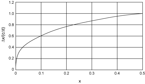Figure 7.7. Curve for selecting weighting parameter x in Muskingum-Cunge method .

Shifts in the Discharge Rating

The stage discharge relationship can vary over time because of changes in the physical features of the gaging station control. If a change in a rating curve stabilizes for a period extending for a month or two, a new rating curve is prepared for the new time period over which the rating curve is effective. If the temporal change is of shorter duration, the original stage discharge relationship is kept; during the period, however, shifts or adjustments are applied to the recorded stage. This is accomplished such that the new discharge represents a recorded stage equal to the discharge from the original rating curve that corresponds to the adjusted stage. The time period over which this occurs is referred to as a period of shifting control.

During periods of shifting control, frequent discharge measurements are essential to identify the stage discharge relation and the magnitude of the shifts during the period. Even with limited data, the rating curve can be estimated if available measurements are supplemented with the behavior of the shifting control. It is this behavior which we will now address.

Detection of Shifts

Rating curves are always subject to minor random fluctuations resulting from the dynamic action of moving water. Rating curves that average measured discharges with relatively close limits are considered acceptable since it is impossible to sort out the minor variations. Moreover, discharge measurements are not error free; an average curve drawn to a set of measurements is more accurate than any single measurement used to define the average curve. A shift obviously occurs when of group of consecutive measurements lies to the right or the left of the average rating curve. This presumes of course that the rating curve is well defined in the range of the current and subsequent discharge measurements. If only one or two measurements depart from the rating curve or a segment of a rating curve, there is no consensus on whether a rating shift has occurred or whether the data represent random error.

Discharge measurements that lie within plus or minus 5 percent of the discharge value of the rating curve are considered to be a verification of the rating curve. If several consecutive measurements satisfy the 5 percent criterion, but they all lie on the same side of a segment of a rating curve, they are considered to define a period of shifting control. If the plus or minus 5 percent criterion is too stringent, departures are acceptable if the indicated shift does not exceed 0.02 feet.

Systematic errors are to be eliminated whenever possible. This can be accomplished by simply changing the measurement conditions as much as possible. For example, the meter or stopwatch can be changed; the measurement verticals can also be changed. If the check measurement agrees with the original rating curve or the current rating trend by 5 percent or less, the original discharge measurement is given no consideration in the rating. It is however entered in the records. If the check measurement verifies by 5 percent or less the original discharge measurement, or the trend in the stage has changed, the two measurements are considered reliable. A single discharge measurement and its check measurement may mark the period of shifting control.

It is also possible to quantify the shift in control using the standard deviation of the stage discharge rating curve. If the rating curve is divided into j segments, the standard deviation of the measurements about the rating curve in the j^th segment, s_j can be computed as

s_j = [∑d_i²/(N-1)]^1/2 7.33

where d_i is the departure of the i^th discharge measurement from the rating curve (percent) and N is the number of measurement used to define the j^th segment of the rating curve.

On the average, 19 out of 20 measurements should depart from the particular rating segment by no more than 2S_j percent. Any subsequent measurement that departs greater than 2S_j are viewed as faulty. The only exception is where two or more consecutive measurements (chronologically or over a range of stage) appear to be well on one side of the plus or minus 2S_j limit. A change in rating curve is required.

In the United States, the statistical approach is not widely used for several reasons. First the limiting criteria of 2S_j percent usually exceeds the 5 percent criteria. Secondly, the statistical approach gives equal weight to all discharge data. More weight should be give to those observations that are rated good to excellent rather than fair to poor. Thirdly, it is generally considered that any subsequent measurement that is verified by a check measurement is more accurate than the rating curve value of discharge.

Rating Shifts in Weirs

Artificial controls are not subject to scour and fill except immediately upstream of the control. Scour will deepen the upstream pool. The approach velocity decreases with the net result that there will be a smaller discharge for a given stage than during the pre-scour conditions. The rating curve will shift to the left of the original rating curve. The opposite situation occurs if there has been deposition or fill.

Scour and fill usually produce minor variations in the rating curve. The shift can be expressed by a parallel shift of the section control portion of the rating curve plotted as a straight line on log paper. Three scenarios are possible for the parallel shift:

there is only a single measurement available; the shift curve is drawn to pass through the measurement
there are several discharge measurements available; the parallel shift curve is drawn to average the discharge measurements, provided there is no indication of a progressive rating shift with time
if the data indicate a progressive rating shift, the shifts are prorated with time. The shift in stage to be applied to recorded gage heights is determined from the vertical distance between the original rating curve and the shift curve.

The time of the shift depends on whether scour or fill has occurred. If fill, the start occurs after the peak discharge of stream rise that precedes the first of the variant discharge measurements. They are started on the recession of the rise. Shifts attributable to scour begin during the high stages of stream rise preceding the first of the variant discharges. The end of the shifts occur on a stream rise that follows the last variant discharge. The general principle is that scour occurs during high stages, and fill occurs during the recession of a stream rise.

The parallel shift of a rating curve implies that for all stages the discharge changes by a fixed percentage. The differences in stage between the two lines increases with stage. Under scour or fill conditions, it is not necessarily true that discharge changes by a fixed percentage. At low flows, there is no impact and the approach velocity is negligible. The impacts of fill or scour on the percentage change in discharge increases rapidly with stage to a maximum value; it then slowly subsides to a percent change that does not differ greatly from the maximum percentage. The parallel shift drawn through these points will fit those relatively large percentage changes in discharge at the higher stage. Conversely at the lower stages, the warped section of the shift curve will adequately fit the rapidly increasing percentage change in discharge. The situation is illustration in Figure 7.8.

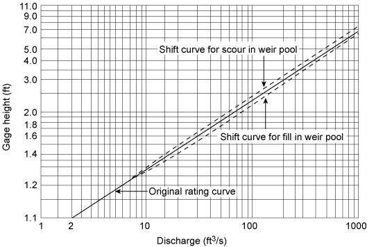Figure 7.8. Rating curve shift due to scour and fill in weir pool.

The approach velocity can also be affected by aquatic vegetation. The approach velocities will be reduced by the increasing friction loss; the rating curve will shift to the left. The shift will however not be abrupt but will gradually increase as the growing seasons continues. The aquatic growth can also impact the weir itself reducing the effective length, b, of the weir. This will also cause a parallel shift of the rating curve to the left on log paper. At all stages, the discharge will be reduced by a percentage equal to the percentage change in effective length of the weir. The shift will either decrease gradually during the vegetation's dormant season, or abruptly if the vegetation is washed out by stream rise.

Moss or algal growth also impact the rating curve. They reduce the head on the weir for any given gage height, G. The head is reduced by the thickness of the growth. The head reduction again shift the rating curve to the left; it is displaced vertically by an amount equal to the thickness of the growth. On rectangular coordinate paper, the shifted rating will be parallel to the original rating. On logarithmic paper, the shifted rating will be convex and asymptotic to the original rating curve.

Rating Shifts in Flumes

Changes in the approach section of flumes most commonly change the stage discharge relation. These changes can occur either in the channel immediately upstream from the flume or in the contracting section of the flume, upstream from the throat. The change is caused by the deposition of rocks and cobbles; removal of the debris restores the original rating curve.

The deposition of debris can divert most of the streamflow to the gage site of the flume; the buildup of water at the gage will shift the rating to the left. The converse situation is also true.

Deposition at the throat entrance of the flume will also cause the rating curve to shift to the left; the stage at the gage is higher than normal for any given discharge. A backwater effect will also results from the growth of algae at the entrance to the throat.

The backwater effect is a decrease in head for a given gage height. It has the effect of increasing the value of e in a linear log plot of the rating curve. The shifted rating curve will be convex and asymptotic to the original rating curve at the higher stages.

Large rocks in high velocity flow events may actually erode the walls and floor of the flume. This increases the roughness and decreases the elevation of the concrete. The two effects tend to compensating. An increase in roughness shift the rating curve to the left; a decrease in elevation, shifts the curve to the rights. In supercritical flumes, the elevation effect predominates.

Rating Shifts in Natural Section Controls

Rating shifts in natural section controls are primarily caused by high velocities associated with high discharges. Boulders, gravel, and sand bar riffles are likely to shift. Following a flood event, the riffles are so dramatically altered that they have no resemblance to pre-flood conditions. A new stage discharge relationship has to be defined for the gaging station. Minor stream rises sort and move the riffle material; their impact on the rating curve is typically a change in the gage height of effective zero flow, e. The shift curve should be defined by current meter discharge measurements. The shift rating on rectangular paper will be parallel to the original rating. The extreme low water portion of the curve can be extrapolated to the actual point zero flow (determined from field measurements). On log paper, the shift will be either convex or concave depending on whether the shift is to the left (increasing e) or the right (decreasing e). In either case, it will tend to be asymptotic to the linear rating at the higher sections of section control.

Vegetal growth in the approach channel has similar effects as discussed in artificial controls. Aquatic vegetation affect the approach velocity; channel growth can reduce the effective length of the control. Aquatic growth on the control will reduce the discharge for any given stage by reducing the head, increasing the flow resistance, and/or reducing the effective length of the control.

Water logged fallen leaves can also clog the interstices and increase the effective elevation of all section controls. This again increases the gage height of the effective zero flow, e.

Rating Shifts in Channel Controls

Natural streams usually have compound controls consisting of channel controls for high flows, and section controls for low flow stages. Scour and fill of the streambed is the most common cause of a shifting channel control. Scour typically occurs during and increase in streamflow, while fill on the recession. Both processes are dependent upon the flow rate (discharge) and the magnitude of the velocity, and the incoming sediment load of the reach. The problem is also complicated in that the length of the channel that is effective as a control is not constant; it increased with discharge.

As a result, there is no substitute for discharge measurements in defining possible shifts in the channel control segment of the rating curve. Of particular importance are measurements made at or near peak stage. Usually, however, a few measurements are available at medium stages; the shifts have to be extrapolated from these data. The results are considered valid if the data conform to the criteria discussed in above.

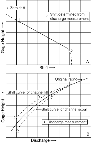
The pattern of scour and fill in a control channel dictates whether the shift increases, decreases, or is relatively constant in stage. A common situation is illustrated in Figure 7.9; here the shift (positive in the case of scour or negative in the case of fill) increases as stage decreases. Graph B of the Figure 7.9 depicts the shift rating corresponding to measurements numbers 1 and 2. The stage shift curve is plotted on rectangular coordinate paper; the rating curves are again represented on log paper. On log paper, the shift curve converge more rapidly toward the original rating curve at the higher stages. The shift curve at the lower stages are shaped to join smoothly with the shift for section control.


Figure 7.9. Channel control rating curve shift.	Figure 7.10. Channel control with increasing rating curve shift as stage increases.

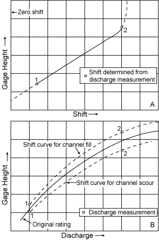
Figure 7.10 depicts the opposite situation where the shifts increase as stage increases. The maximum value of the shift is only slightly greater than the maximum observed value. This is done to prevent overcorrecting the original rating curve. The period associated with the shifting control corrections is terminated on the stream rise following the last shift measurement; the original rating is used on the rising limb of the rise.

Scour in channel control produces a positive shift because the depth, and as a result discharge, is increased for a given gage height. Deposition results in a minus shift; depth and therefore discharge are decreased for a given gage height. The discharge effect of scour and fill is opposite to that occurring in a weir pool. Recall that in a weir, these processes affect only the approach velocity. If a permanent weir is a part of the compound control, scour in the weir pool and the channel control will produce a negative shift in the section control rating; a positive shift will result for the channel control.

Shift in the rating curve are also caused by variation in the width the stream channel. Even in relatively stable channels, channel width may be increased during intense floods by bank cutting. In north coastal California, channel widths are also reduced by frequent landslides that occur when steep streambanks are undercut. The impact on the rating curve of a change in the channel width is to change the discharge by a fixed percentage for a given gage height. This assumes there is no change in the streambed elevation. The original model of the rating curve is

Q=p(G-e)^N 6.2

and when plotted on log paper is a linear equation. As the width changes, the value of p increases with increasing channel width and decreases with decreasing width. The shift curve associated with the change in the channel width will be parallel to the rating curve on log paper. A single discharge measurement is sufficient for identifying the shift curve for the channel control.

If a change in streambed elevation occurs, the impact of both the width and elevation changes is complex. It requires at least several discharge measurements to define the shift curve.

Vegetal growth also affects the stage discharge relationship. It effectively reduces the discharge for a given gage height. The shift rating will plot to the left, a minus shift, or the original rating curve. The vegetation increases the roughness of the channel and constricts the unobstructed channel width. Both factors reduce the value of p in Equation 6.1. If the change in the roughness and effective width are unchanging with stage, the shift curve will be parallel to and to the left of the original rating curve. More commonly, however, these changes are not independent of stage. The rating shift associated with vegetation is variable in time as the vegetation spreads and increases in size.

Procedures for Shift Adjusting Ratings

The preceding discussion focused on the processes that lead to rating shifts and how shifts are recognized. This section will describe typical procedures for defining a shift and incorporating it into a rating curve to produce a shift adjusted rating. The relevance of these procedures to operational hydrology will be illustrated.

Once a sequence of paired stage/discharge measurements indicate that a change in the relationship between stage and discharge over some range of stage values, a new rating curve is drawn. The new curve incorporates the shift in relevant portion of the rating and the original unshifted portion of the official rating curve. The new curve would only be used by the hydrologist performing the analysis to develop a shift adjusted rating. An example of a hand drawn curve that incorporates a shift is shown in Figure 7.11.

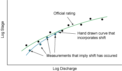Figure 7.11. Rating curve with a hand drawn shift.

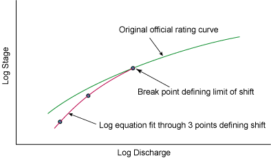
Three points on the hand drawn shift curve are typically chosen to characterize the shift. Figure 7.12 shows an example of how these points would be selected. The points are reported as an input, or discharge for which the shift occurs, and the shift, or difference between the official rating and the shifted curve. The values of the input and shift are used to communicate the nature of the shift. These data pairs are provided by the USGS on official rating tables, as shown in Table 6.1. The data pairs associated with the shift in Figure 7.12 are shown under the rating curve plot.

Figure 7.12. Rating curve with three defining points selected from the hand drawn shift .

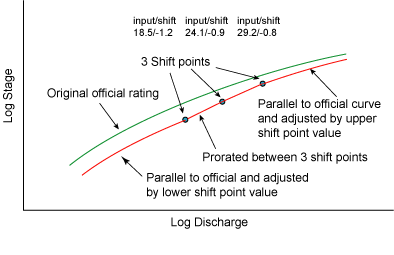
Once the three defining points are selected, a new logarithmic function is determined that passes through these three points. Values are extracted from this function every 0.01 feet to produce a shift adjusted rating table. For stages beyond the influence of the shift, the existing, unshifted, rating values are used as shown (Figure 7.13).

Figure 7.13. Rating curve with a shift defined by a logarithmic function.

The shift curves shown in Figures 7.11 through 7.13 converge with the original rating curve because the effect of the shift diminishes with increasing stage until the shift is not detectable. for the example illustrated, the convergence of the two rating curves is quantifiable because enough measurements were available to define the shift throughout the range of stages for which it applies. The ability to obtain a sufficient number of measurements to define the entire shift is common for low and moderate flow shifts, since low and moderate flows frequently occur providing ample safe sampling opportunities.

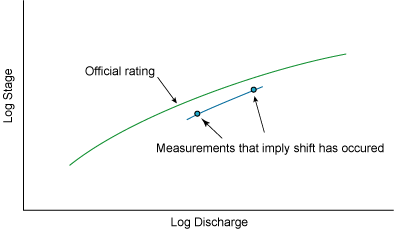
Adequately defining the entire range of a high flow shift is frequently difficult due to the infrequency of high flows and the difficulty of taking high flow discharge measurements. Figure 7.14 illustrates a shift occurring for high flow. In this case, measurements are not available to define the high end of the shift. The shift is characterized by prorating the values between the three defining points and extracting rating values at 0.01 foot increments. For stages above the shift, the original rating values are used after they are adjusted by the amount of the shift associated with the highest stage. The original rating curve and the shift adjusted curve would therefore be parallel in rectangular coordinates above the last shift point. If Figure 7.15, these curves are shown as nearly parallel for illustrative purposes but in log coordinates, they would appear to converge. The same approach is applied to develop rating values below the shift point associated with the lowest stage if lower flow measurements are not available to define the lower portion of the shift.

Figure 7.14. Rating curve with a hand drawn high flow shift.

Figure 7.15. High flow shifted rating curve.

The data pairs used to describe shifts provide useful insight into the nature of the shift. This insight can be valuable to river flood forecasters. The input values indicate the range of stages for which the shift is occurring. When these are compared to the range of stages possible for a site during a runoff event, it can quickly be assessed whether the shift impacts low flow or high flow conditions, and also whether the shift impacts stages of concern, such as Flood Stage. The real value in the shift data pairs, however, is in their ability to convey whether a shift is fully documented.

Recall that the shift described in Figures 7.11 through 7.13 converges with the official rating at moderate flows. This is revealed in the shift data pairs by the fact that the shift diminishes to zero. Conversely, the nature of the shift in Figures 7.14 and 7.15 is not known at high flows. This can be seen in the shift data pairs because the shift values do not trend to zero at high stages. The implication of this to flood forecasting is that the magnitude of the shift at high flow estimated with considerable uncertainty. The shift uncertainty results in additional uncertainty in the transformation from forecasted flow to forecasted stage that could have a significant impact on the final accuracy of a river forecast.

NWS operational hydrologist typically do not have access to the hand drawn curves used to characterize and track rating shifts. Furthermore, the rating table values do not reveal any insight into the nature of any incorporated shift, and rating curves plotted on computer monitors frequently mask the shift. Therefore it is important for the hydrologists to examine the shift data pairs which are published on the rating curve to be able to assess the nature of shifts.

Lesson 7 Summary

In practice, ratings curves are often extended or extrapolated beyond the range of observed discharge measurements. The extrapolation of the rating data can lead to considerable uncertainty in the prediction of discharge. This lesson examined low flow and high flow extrapolation techniques, the processes responsible for rating curve shifts, and methodologies quantify and accommodate possible shifts in the stage discharge relationship.

The following terms and concepts were introduced in this lesson and should be mastered prior to continuing with on to Lesson 8. Selecting a link in the list below will result in a jump to the portion of the lesson material above that covered the relevant material so that it can be reviewed as necessary.

Definitions
Concepts

Lesson 7 Review Questions

The slope-area method is used to:
The uncertainty associated with the high end of a rating curve results from:
Agencies, such as the USGS, that maintain rating relationships frequently develop a new official rating once enough measurements have been taken to fully define a shift.
- True
- False

Lesson 8 Preview

The discharge rating curve transforms the stage data to a continuous record of stream discharge. In some situations, the discharge may be determined by stream stage alone (see Lesson 6). However, in an unsteady flow situation, the energy slope of the stream changes with the stream stage. As a result, the stage discharge relationship can not be uniquely determined by stream stage alone. Lesson 8 examines complex stage discharge models in which the discharge is not a function of stage only.